Monte Carlo Simulation using Python

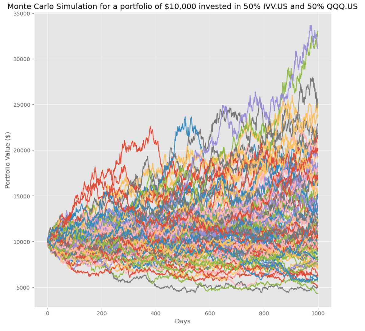
Here is an example project to use Python, Pandas, Numpy and Matplotlib to perform a Monte Carlo Simulation for an investment portfolio of investing in 2 stocks namely IVV.US and QQQ.US, by running a simulation of 1000 scenarios:

1
2
3
4
5
6
7
8
9
10
11
12
13
14
15
16
17
18
19
20
21
22
23
24
25
26
27
28
29
30
import pandas as pd
import numpy as np
import matplotlib.pyplot as plt

ivv = pd.read_csv(r".\financial_data\IVV_US.csv")
qqq = pd.read_csv(r".\financial_data\QQQ_US.csv")

ivv.tail(2)

Date Open High Low Close Adj Close Volume
6011 2024-04-12 516.929993 518.349976 511.600006 513.309998 513.309998 6512900
6012 2024-04-15 517.690002 517.809998 506.049988 506.950012 506.950012 6397300

qqq.tail(10)

Date Open High Low Close Adj Close Volume
6315 2024-04-16 430.899994 433.760010 429.700012 431.100006 431.100006 47619000
6316 2024-04-17 433.100006 433.119995 424.899994 425.839996 425.839996 56880500
6317 2024-04-18 426.489990 428.239990 422.829987 423.410004 423.410004 46549400
6318 2024-04-19 422.220001 422.750000 413.070007 414.649994 414.649994 75136600
6319 2024-04-22 417.309998 421.179993 413.940002 418.820007 418.820007 47807700


# merge 2 tables:
merged_close = pd.merge(ivv, qqq, on='Date',suffixes=['_ivv', '_qqq'])[['Date', 'Close_ivv','Close_qqq']]

# set date column to the index:
merged_close['Date'] = pd.to_datetime(merged_close['Date'])
merged_close.set_index('Date', inplace = True)

Calculate daily returns and mean returns and Compute pairwise covariance

1
2
3
4
5
6
7
8
9
10
11
12
13
14
# get the daily returns and mean returns
returns_close_prices = merged_close.pct_change()
mean_returns = returns_close_prices.mean()

# Compute pairwise covariance of for the daily returns for both IVV and QQQ
covMatrix_close_prices = returns_close_prices.cov()

covMatrix_close_prices

>> result:
Close_ivv Close_qqq
Close_ivv 0.000147 0.000172
Close_qqq 0.000172 0.000274

Perform Monte Carlo Simulation for 1000 days investment time frame with 1000 scenarios

1
2
3
4
5
6
7
8
9
10
11
12
13
14
15
16
17
18
19
20
21
22
23
24
25
26
27
28
29
30
31
32
33
34
35
36
37
38
39
40
#generate random weights for the portfolio allocations to each stocks:
weights = np.random.random(len(mean_returns))
# Normalizing the Weights: To ensure that the weights sum up to 1
weights /= np.sum(weights)

# number of simulations
num_of_sims = 100
# timeframe in days
t_days = 100

num_holdings= len(weights)

# Creates a matrix of shape (t_days, num_holdings) where each entry is filled with the mean returns of the assets.
mean_matrix = np.full(shape=(t_days, num_holdings), fill_value=mean_returns)

# Transposes the mean returns matrix to shape (num_holdings, t_days) to match the dimensions required for later calculations.
mean_matrix = mean_matrix.T

# Initializes an empty matrix to store the results of the portfolio simulations. The matrix has t_days rows and num_of_sims columns.
portfolio_sims = np.full(shape=(t_days, num_of_sims), fill_value=0.0)

inital_value = 10000

# Loops over the number of simulations:
for m in range(0, num_of_sims):
# Draw random values from a normal distribution. This matrix simulates daily returns for each asset over the specified timeframe.
z = np.random.normal(size=(t_days, num_holdings))
# Computes the Cholesky decomposition of the covariance matrix of the asset returns, to introduce correlations between the random returns.
l = np.linalg.cholesky(covMatrix_close_prices)
# Calculates the daily returns for each asset by adding the mean returns to the product of the Cholesky decomposition
# and the random normal variables. This is where the correlation between asset returns is applied.
daily_returns = mean_matrix + np.inner(l, z)
portfolio_sims[:,m] = np.cumprod(np.inner(weights, daily_returns.T) + 1) * inital_value

plt.plot(portfolio_sims)
plt.ylabel('Portfolio Value ($)')
plt.xlabel('Days')
plt.title('Monte Carlo Simulation of a stock portfolio with investing of ')
plt.show()